LCS is a library for performing Lagrangian coherent structure (LCS) analysis of flow field. OpenMP is supported for parallelization.

It implements particle advection calculations for both discrete and continuous flow velocity data, and then uses finite-time Lyapunov exponent technique to obtain LCSs.

Suppose we have the flow map $\phi(t_0+T,\mathbf{x}_0,t_0)$ obtained after fluid particle advection, where $\mathbf{x}_0$ and $t_0$ are intial particle position and time, and $T$ is the advection time (integration time). Then, FTLE is defined as

$FTLE(\mathbf{x}_0,t_0) =\frac{1}{2T}\log\Big\{\lambda_{\max}\Big[\Big(\frac{\partial\phi}{\partial\mathbf{x}_0}\Big)^T\Big(\frac{\partial\phi}{\partial\mathbf{x}_0}\Big)\Big]\Big\},$

where $\lambda_{\max}$ denotes the maximum eigenvalue of a matrix. Here, the matrix is called Cauchy-Green tensor.

Installation and Running

First, clone the repository from Gitub and enter the repository folder:

git clone https://github.com/stevenliuyi/lcs

cd lcs

Please make sure that your compiler supports C++14 standard, and then compile the program:

make

The compiled programs will be in the bin folder. There are two demo programs demo_continuous_double_gyre and demo_discrete_double_gyre, for continous and discrete data respectively. Please refer to the examples below for more details. You could run the program as:

bin/demo_continuous_double_gyre

If you'd like to change the threads for OpenMP, you could set the environment variable OMP_NUM_THREADS.

The demo result files are double_gyre_ftle_pos.txt and double_gyre_ftle_neg.txt, for positive FTLE (forward advection) and negative FTLE (backward advection) respectively.

Plotting

There is no graphics support in the program, but you could easily make plots in other programs with the result data files. For example, the contour FTLE plots below shown in the examples can be easily generated in python as:

 import numpy as np
 import matplotlib.pyplot as plt
 
 ftle = np.genfromtxt('double_gyre_ftle_neg.txt', skip_header=3).reshape((1000,500))
 x = np.linspace(0,2,num=1000)
 y = np.linspace(0,1,num=500)
 X, Y = np.meshgrid(x, y, indexing='ij')
 plt.contourf(X, Y, ftle, 100, cmap=plt.cm.Reds)
 plt.show()

Examples

Continuous data

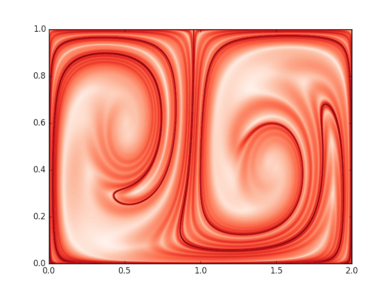
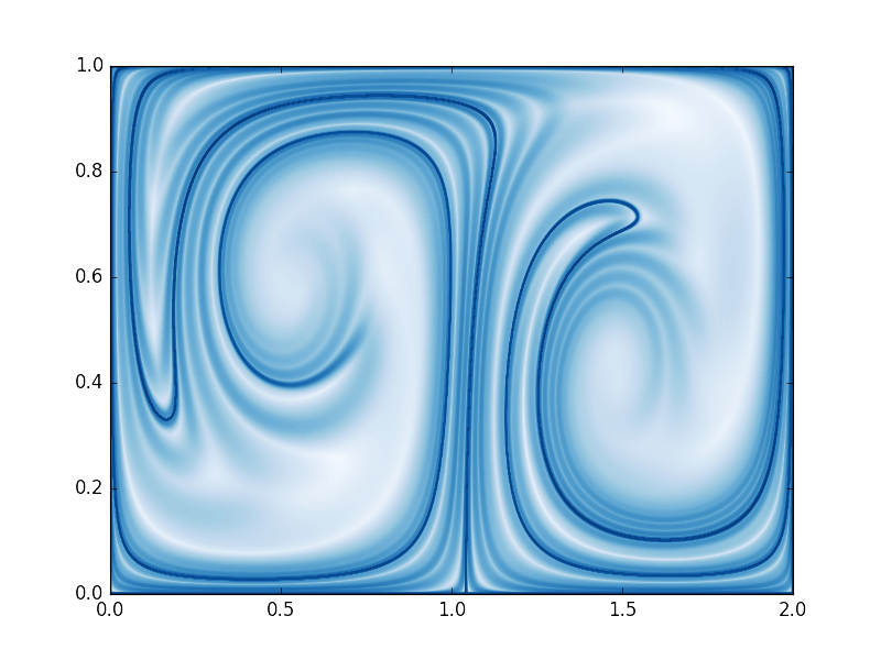
Here we show a demo of perform FTLE calculation for a double-gyre model. The implementation is included in continuous_double_gyre.cpp.

pFTLE	nFTLE

First, we create a ContinuousFlowField object, and set the grid shape as $(1000,500)$ , the range of $x$ -coordinate as $(0,2)$ , and the range of $y$ -coordinate as $(0,1)$ . Note that this is a 2D flow field, so we should set the dimension to be 2 for the object.

ContinuousFlowField<double,VelocityFunction::DoubleGyreModel<double>,2> double_gyre(1000,500);

double_gyre.InitialPosition().SetAll(0,2,0,1);

Next, we set each integration time step as $\Delta t=0.1$ , and the number of steps as $n=200$ :

double_gyre.SetDelta(.1);

double_gyre.SetStep(200);

Now we have done all the settings, and we could then simply advect the particles to obtain the flow map:

double_gyre.Run();

Finally, we could calculate FTLE based on the flow map we just obtained:

FTLE<douuble,2> ftle(double_gyre);
ftle.Calculate();
ftle.WriteToFile("double_gyre_ftle_pos.txt");

If we would like to obtain the flow map in backward direction and then calculate the negative FTLE corresponding to it, we could simply flip the advect direction and redo the calculations as:

double_gyre.SetDirection(Direction::Backward);
double_gyre.SetInitialTime(20);
double_gyre.Run();
ftle.Calculate();
ftle.WriteToFile("double_gyre_ftle_neg.txt");

Discrete data

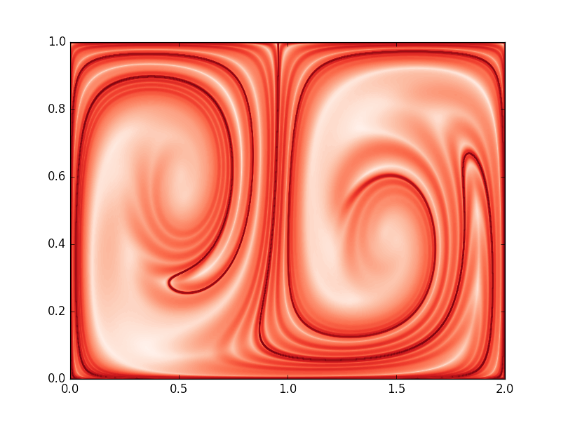
Normally, discrete velocity data are obtained from experiments or CFD simulations. But here we will use the discrete data genereted by the analytic velocity function in the above example, so we could directly compare the results.

The implementation is included in discrete_double_gyre.cpp.

pFTLE	nFTLE

First, we use the double-gyre velocity function to generete velocity data at $t=0,1,2,\cdots 20$ with 100 grid points in $x$ -direction and 50 grid points in $y$ -direction.

Position<double,2> pos(100,50);
pos.SetAll(0,2,0,1);
ContinuousVelocity<double, VelocityFunction::DoubleGyreModel<double>,2> double_gyre_vel(100,50,pos);
for (int t=0; t <= 20; ++t)
{
    std::stringstream ss;
    ss << "double_gyre_" << t << ".txt";
    double_gyre_vel.UpdateTime(t);
    double_gyre_vel.SetAll();
    double_gyre_vel.WriteToFile(ss.str());
}

Next, we create a DiscreteFlowField object with the same grid shape and $x$ -, $y$ -range as in the continuous data example. Note that we also need to set the grid shape of the velocity data to be $(100,50)$ , as we defined above.

DiscreteFlowField<double,2> double_gyre(1000,500,100,50);
double_gyre.DataPosition().SetAll(0,2,0,1);
double_gyre.InitialPosition().SetAll(0,2,0,1);

To correctly read the velocity data, we also need to define the format of the file names:

double_gyre.SetVelocityFileNamePrefix("double_gyre_");

Now we can set the integration time step and the number of steps as before, but for discrete data, we also need to set the time step between two adjacent data files, as well as the total time range all data files cover:

double_gyre.SetDataDelta(1);
double_gyre.SetDataTimeRange(0,20);
double_gyre.SetDelta(.1);
double_gyre.SetStep(200);

Now we can advect the particles and calculate FTLE:

double_gyre.Run();
FTLE<douuble,2> ftle(double_gyre);
ftle.Calculate();
ftle.WriteToFile("double_gyre_ftle_pos.txt");

We can also calculate negative FTLE the same way as we did in the continous data example.